MARKETICA_PREVIEW/00-marketica-preview-sale37.jpg
MARKETICA_PREVIEW/01_marketica2_homepage.png
MARKETICA_PREVIEW/02_marketica2_shop_page.png
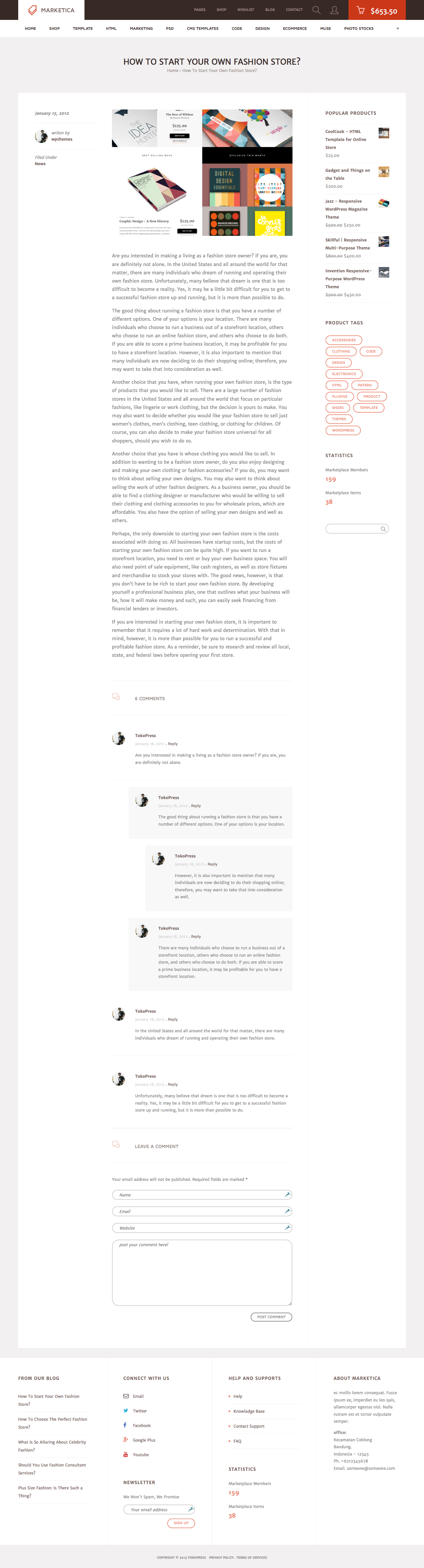
MARKETICA_PREVIEW/03_marketica2_single_product_page.png
MARKETICA_PREVIEW/04_marketica2_cart_page.png
MARKETICA_PREVIEW/05_marketica2_checkout_page.png
MARKETICA_PREVIEW/06_marketica2_myaccount_login_page.png
MARKETICA_PREVIEW/07_marketica2_plan_and_pricing_page.png
MARKETICA_PREVIEW/08_marketica2_team_members_page.png
MARKETICA_PREVIEW/09_marketica2_contact_page_template.png
MARKETICA_PREVIEW/10_marketica2_blog_page.png
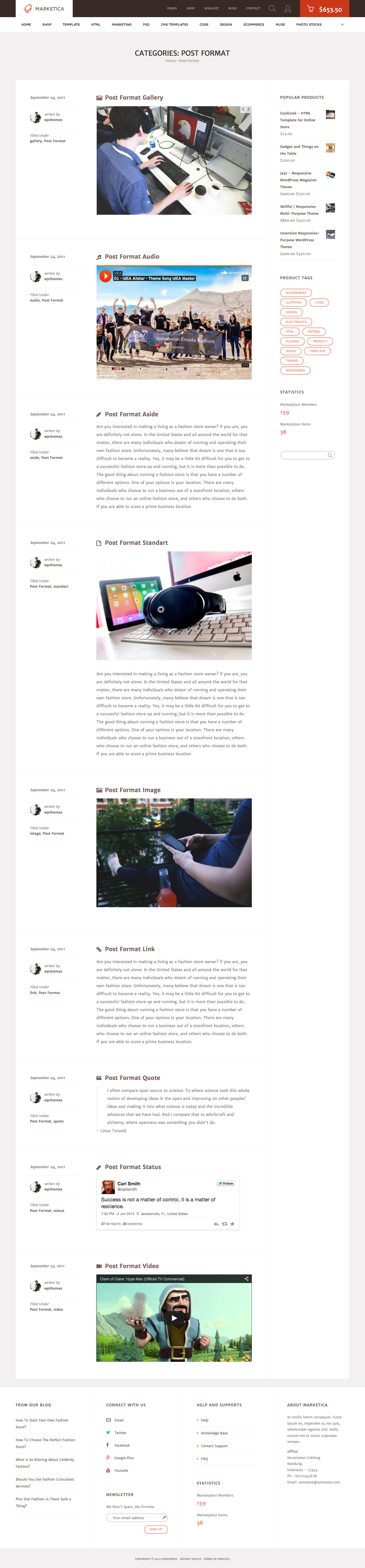
MARKETICA_PREVIEW/11_marketica2_blog_post_formats.png
MARKETICA_PREVIEW/12_marketica2_single_product_page.png
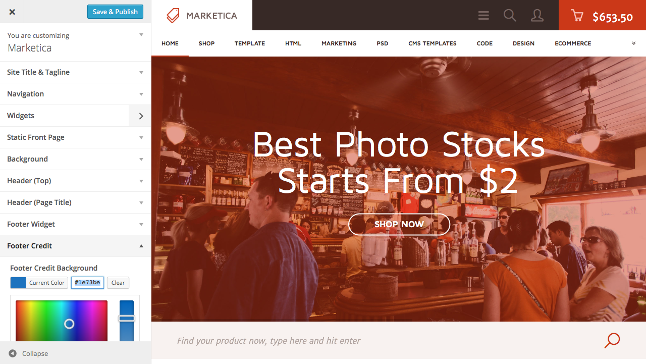
MARKETICA_PREVIEW/13_marketica2_theme_customizer.png
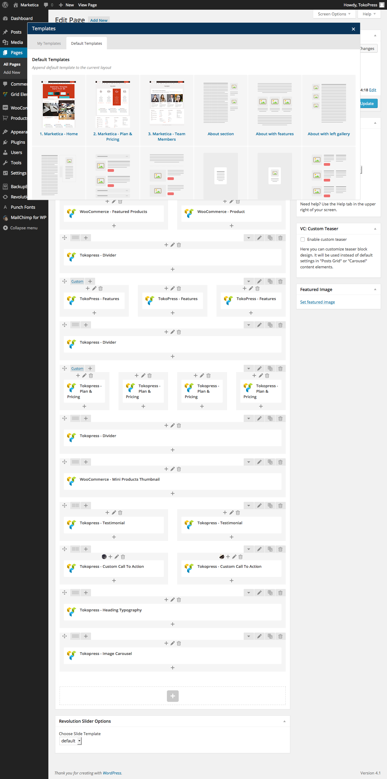
MARKETICA_PREVIEW/14_marketica2_visualcomposer_templates.png
MARKETICA_PREVIEW/15_marketica2_tablet_view.png
MARKETICA_PREVIEW/16_marketica2_tablet_view_offcanvas_menu.png
MARKETICA_PREVIEW/17_marketica2_themeoptions_header.png
MARKETICA_PREVIEW/18_marketica2_themeoptions_footer.png
MARKETICA_PREVIEW/19_marketica2_themeoptions_contact.png
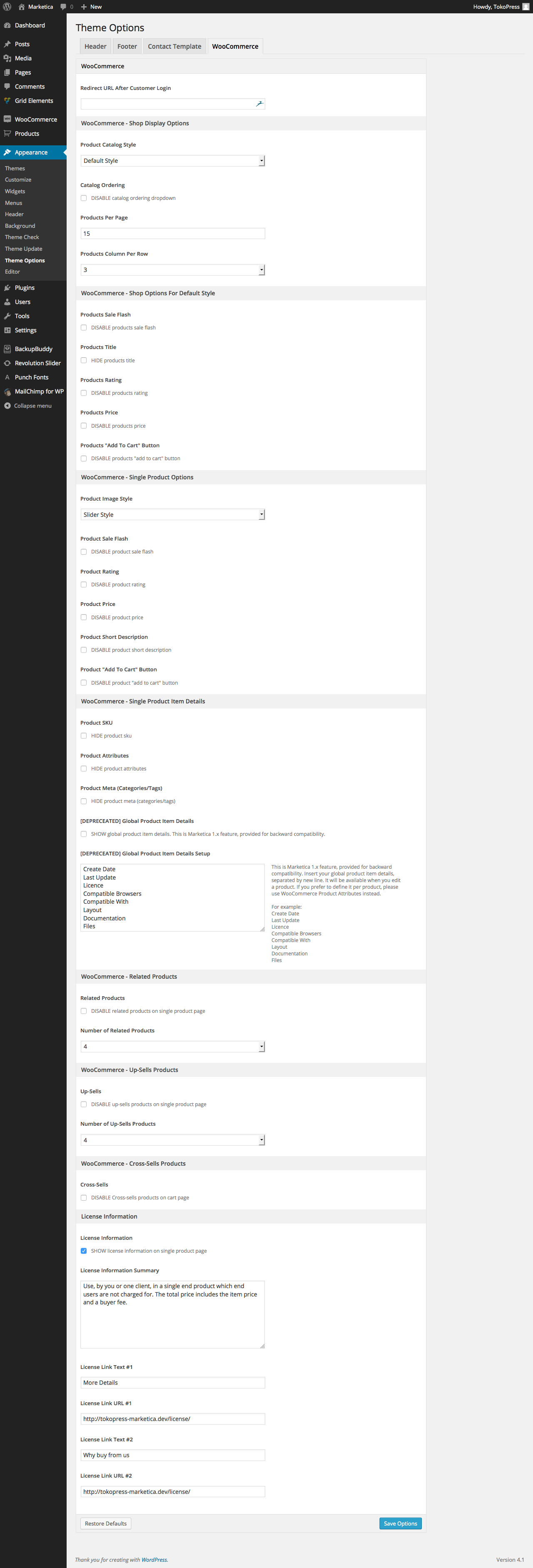
MARKETICA_PREVIEW/20_marketica2_themeoptions_woocommerce.png
MARKETICA_PREVIEW/21_marketica2_wcvendors_user_page.png
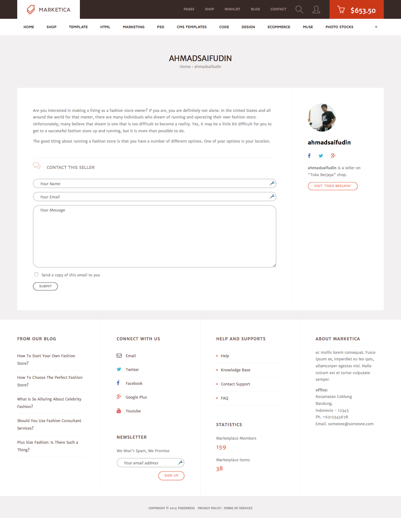
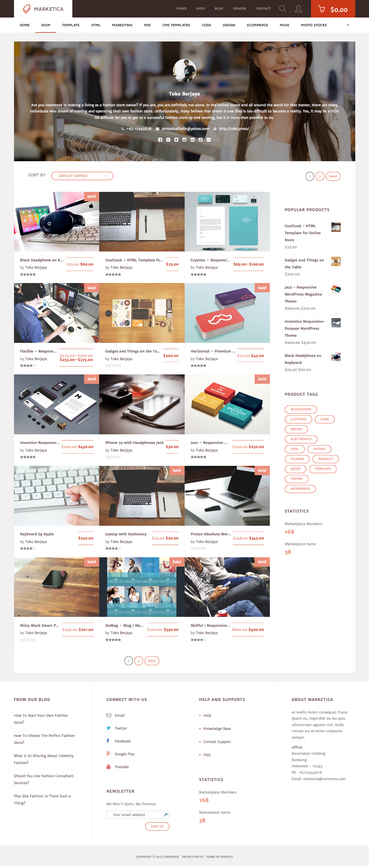
MARKETICA_PREVIEW/22_marketica2_wcvendors_vendor_page.png
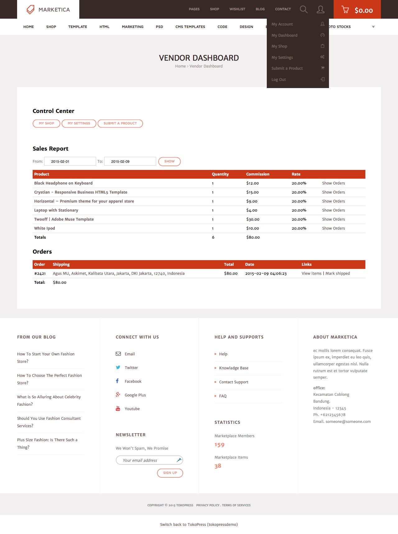
MARKETICA_PREVIEW/23_marketica2_wcvendors_vendor_dashboard.png
MARKETICA_PREVIEW/24_marketica2_wcvendors_shop_settings.png
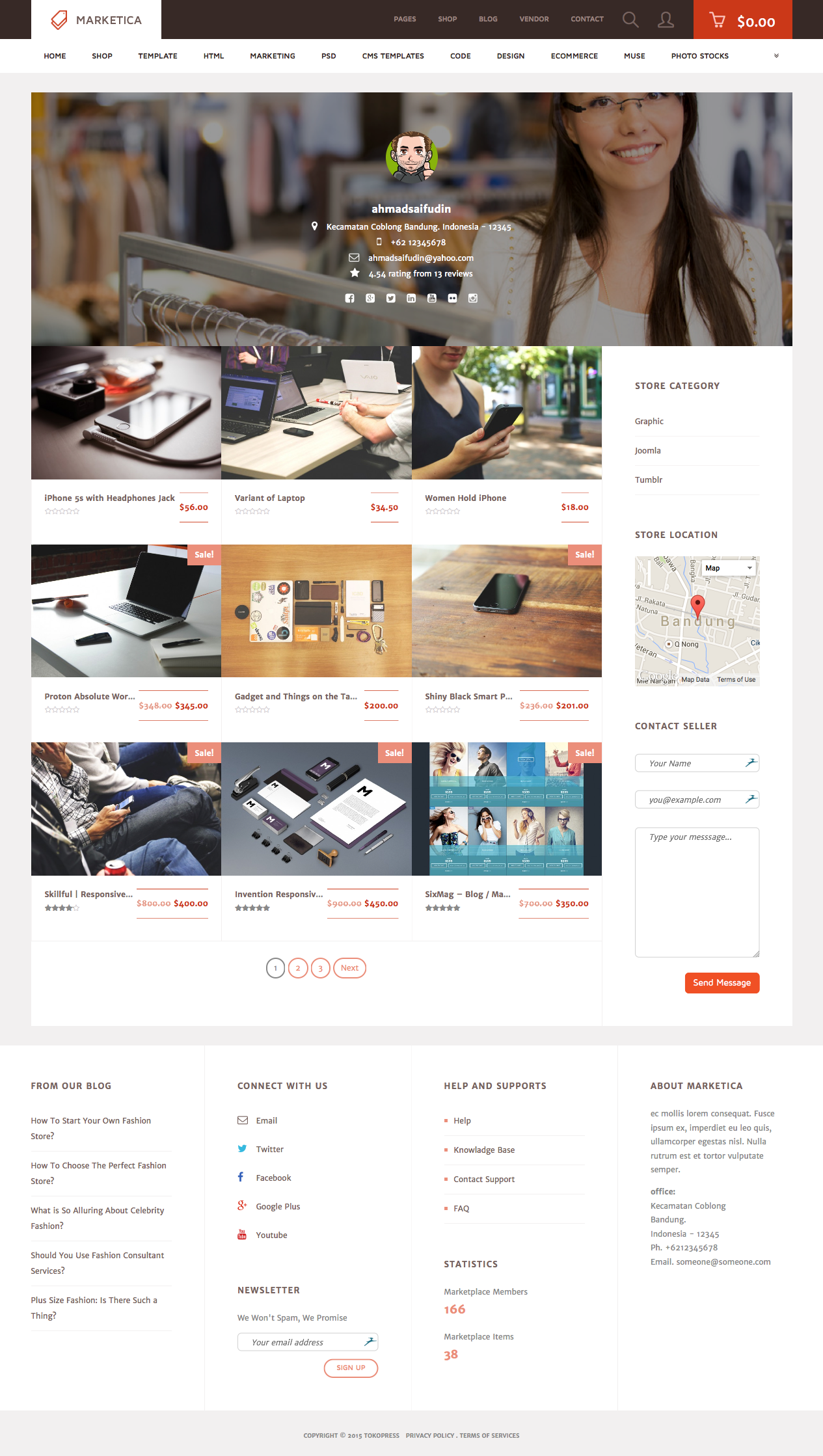
MARKETICA_PREVIEW/25_marketica2_dokan_vendor_store_page.png
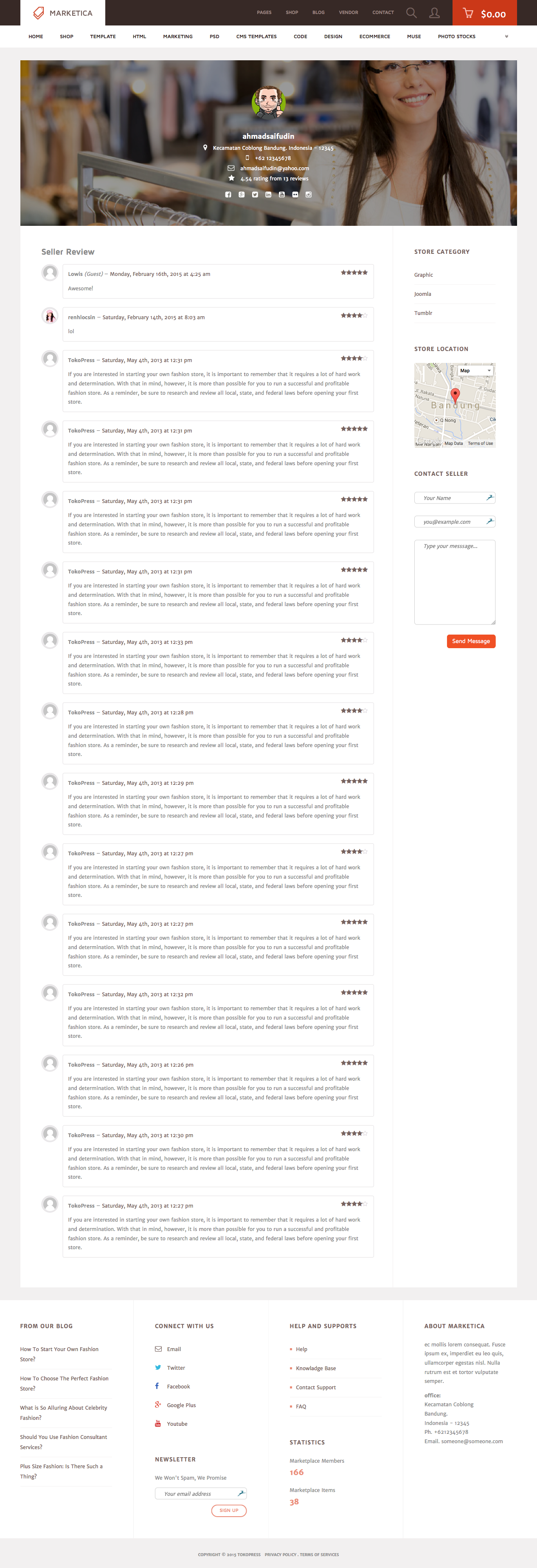
MARKETICA_PREVIEW/26_marketica2_dokan_vendor_review_page.png
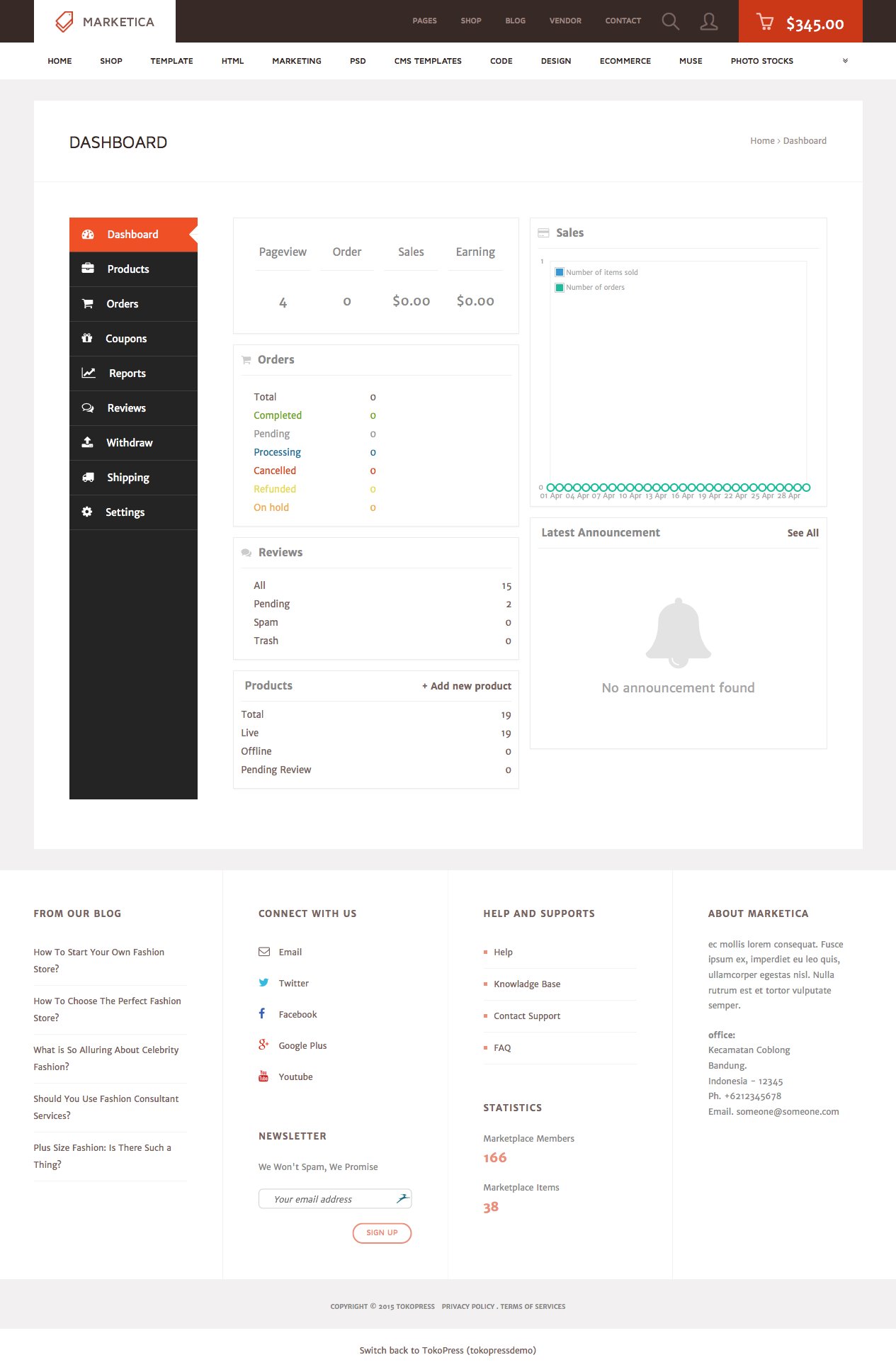
MARKETICA_PREVIEW/27_marketica2_dokan_vendor_dashboard_page.png
MARKETICA_PREVIEW/28_marketica2_dokan_vendor_dashboard_products_page.png
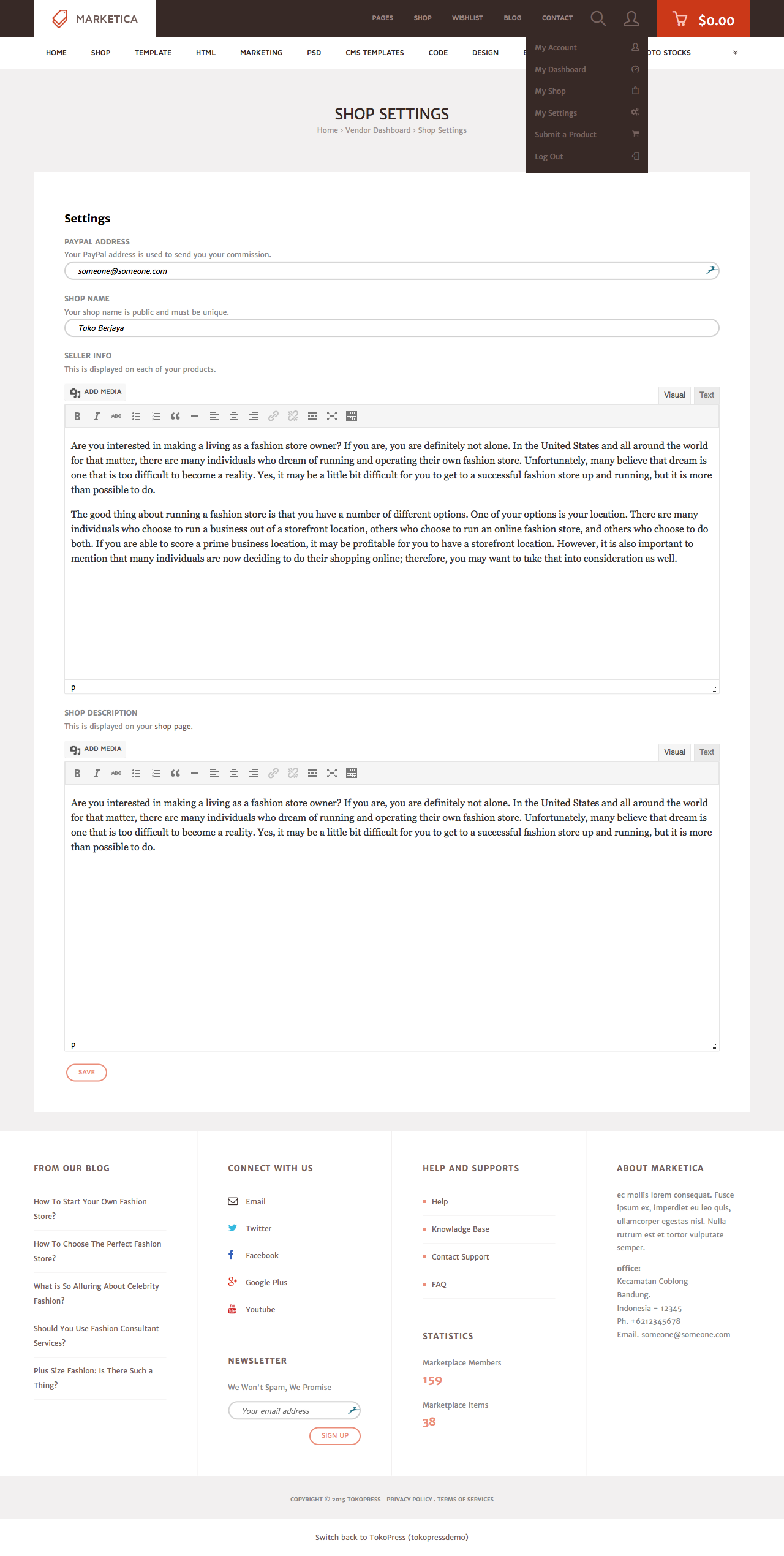
MARKETICA_PREVIEW/29_marketica2_dokan_vendor_dashboard_settings_page.png
All Rights Reserved Rk77
Rk77
Rk77
Rk77 > Login Game Apk Thailand Versi 12.02Mb Android Mobile Download Mudah Anti Blokir
Rk77 Game Berlesensi
Rk77 menghadirkan aplikasi game Thailand berukuran 12.02Mb yang ringan dan mudah dipasang pada perangkat Android. Proses login dirancang praktis dengan sistem akses yang stabil serta dukungan fitur anti blokir. Tampilan sederhana memudahkan navigasi, sementara pembaruan berkala membantu menjaga performa aplikasi agar tetap responsif dan nyaman digunakan kapan saja.
Rk77 Apk Download Gratis Tanpa VPN
Rk77 Menghadirkan Sebuah Aplikasi Resmi Berlisensi Dengan Link Download Gratis Super Premium, Tanpa Iklan Install Lebih Cepat, Serta Ukuran File Yang Lebih Ringan Dan Unduh Tanpa VPN.
 PROMO
PROMO
 LOGIN
LOGIN
 DAFTAR
 WHATSAPP
 Live Chat